Category Archives: Electronics

Painbox part 3: a bunch of updates

Since I last wrote about my Painbox project (part 1, part 2), progress has been very lumpy. Here’s a bunch of short updates on various aspects of the project.

The grill

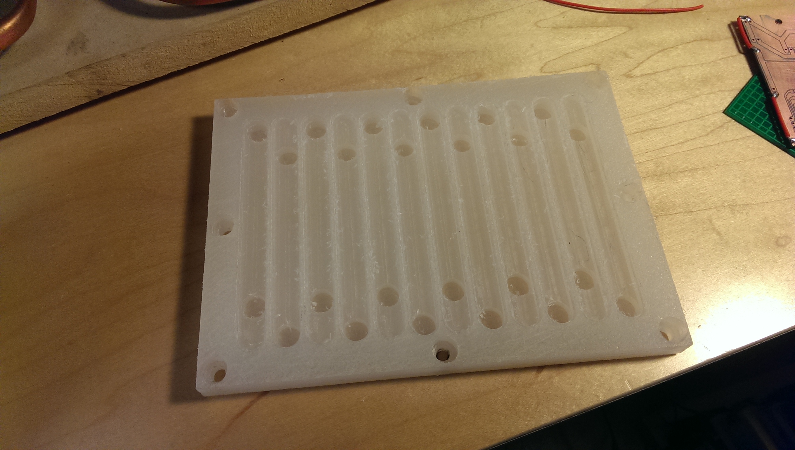
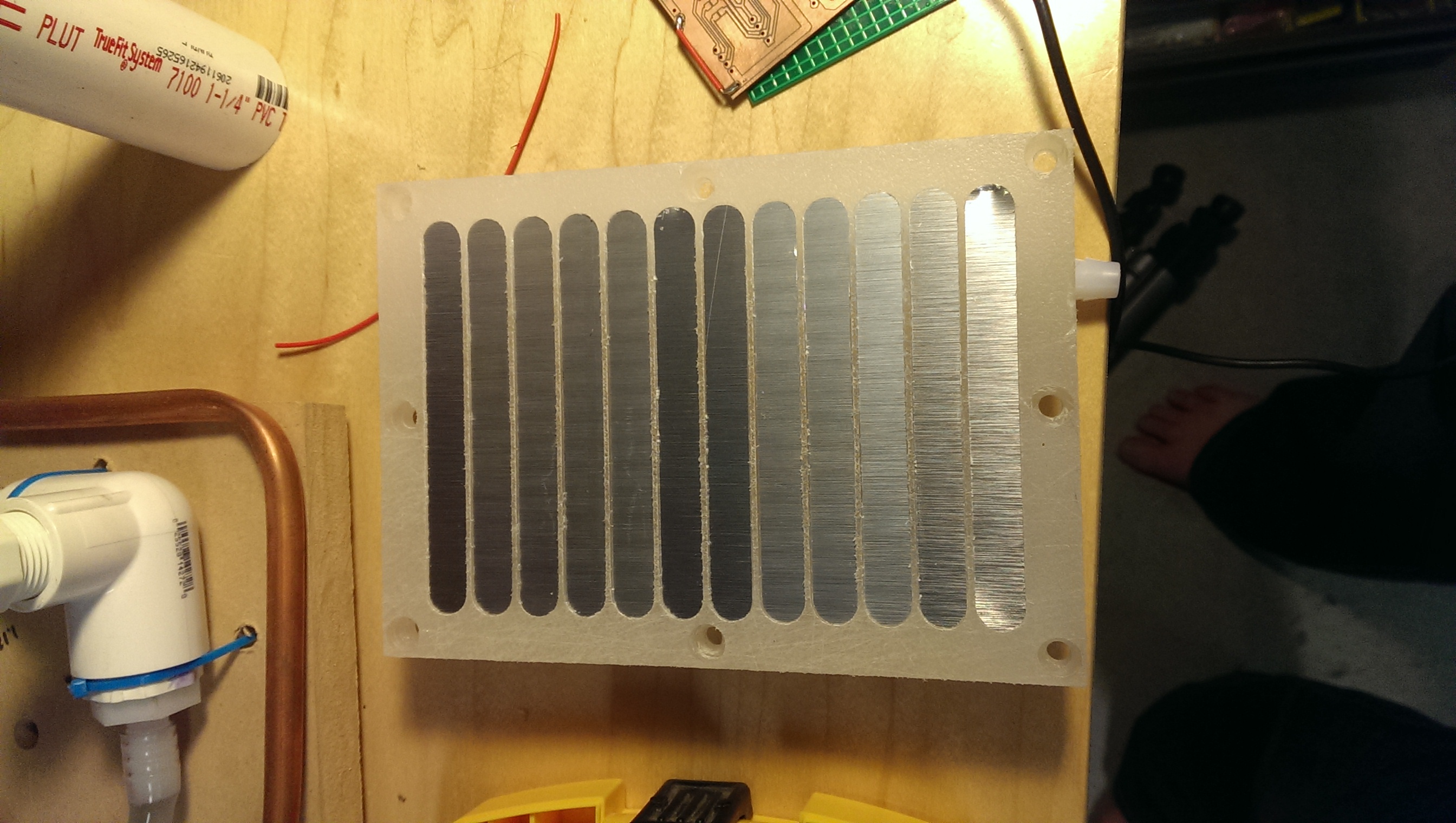Replacing the clunky “copper tubes through a 2×4″ test grill was high on my list of priorities, so I tackled that first. I considered a number of different options, but settled on making a custom one-piece grill out of a 1/2″ HDPE cutting board. Essentially, it’s like a two-sided PCB, except instead of copper traces and plated vias, I milled width-wise grooves into the top and length-wise grooves into the bottom with through-and-through holes connecting the two sides. The result is a sort of channel that snakes across the top, through to the bottom, over the neighboring groove, then back to the top. To make it capable of moving water, I capped the grooves with pieces of 0.025” aluminum sheet, also cut out on the Shapeoko 2. The first and last hole of each path are threaded to accept a hose barb.

Other than the capping and sealing process, which was awkward and imprecise, the whole thing turned out really good. If I was going to do it again, I would use a piece of virgin HDPE instead of a cutting board so it would have a better surface finish. I’d also probably go with thicker stock, since that would improve durability and flatness while increasing the margin for error during machining.

Temperature sensors and reservoir design

In the last post, I talked about my success with immersing the sensors directly in the water. To try and make that more permanent, I drilled a small hole in the top of my reservoir caps, threaded a thermistor through the hole, and then tried to seal the whole thing up with some silicone glue stuff I had lying around.

This did not work.

Problem 1 – the water in the reservoirs does not really reach the thermistor, since they are not hanging down that low, and the water is not that high. Result: bad readings.

Problem 2 – the silicone stuff is glue, not epoxy or sealant. While it appears to solidify into a rubbery plug, it turns out it really doesn’t like to cure solid when it’s in a big blob, and over time gravity will let it goop down and into the moving water, where it will ultimately foul your pump. I had to disassemble and clean out one of my aquarium pumps four times before I realized there was probably a loose blob trapped elsewhere in the system. Turned out it was hanging on to the fins inside the water block and would occasionally throw a clot or two after an hour of continuous running. After cleaning that out, problem solved.

Problem 3 – trying to keep things simple, the connection style is just a long wire pair soldered to the thermistor. When manipulating the reservoir cap, that long wire wants to twist up unless it’s disconnected from the microcontroller, and even once it’s disconnected, it flops all over the place while you’ve got a wrench on it, making it pretty unwieldy.

A related problem is that my reservoirs just don’t work that well. I’d previously decided to make them small so that there’d be less water volume in the system, but somehow at the same time I ended up with reservoirs that made it hard to fill or drain the whole system. Water just didn’t want to disseminate into the system when added to the tiny reservoir.

Combined with the temp sensor issues, this lead me to change my reservoir design. Instead of a 3-way corner elbow, I’m using a 4-way tee as the base and adding appropriate threaded connectors and hose barbs. The inlet and outlet will be oriented such that the water will flow downward from the inlet to the outlet. Across from the inlet, I’ve added a dedicated port for the thermistor, which will still be connected to a threaded cap. However, this time I’m going to try to drill individual holes for each of the thermistor’s leads and use a minimum amount of actual sealant to make it waterproof. Since the sensor will now be level with the inlet, I can just fill the reservoir until the inlet is covered and know the sensor will also be immersed. With the legs exposed on the outside, I’ll solder a tiny connector board on that allows for easy disconnection. The final branch of the 4-way tee will be the fill port, which will just have a plain cap in it. I might add a bleed valve of sorts to the top of the fill cap if I find the system needs help shedding bubbles.

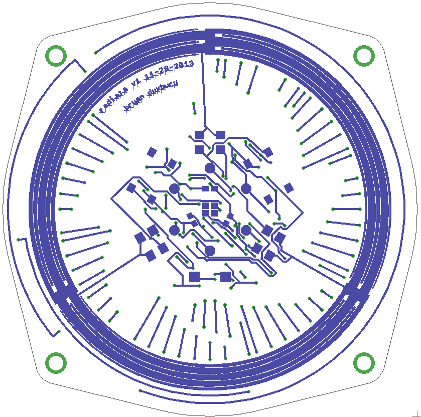
TEC controller board

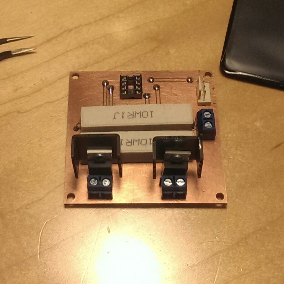
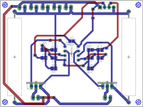
Latest version of the TEC controller

During earlier testing, I didn’t use any sort of closed-loop control scheme, which lead to, well, uncontrolled temperatures. To implement closed-loop control in this system, you need a sensor, a TEC controller, and the logic to control it. For the sensor, I’m using the aforementioned thermistors. The logic part is easy, and comes in the form of an Arduino PID library.

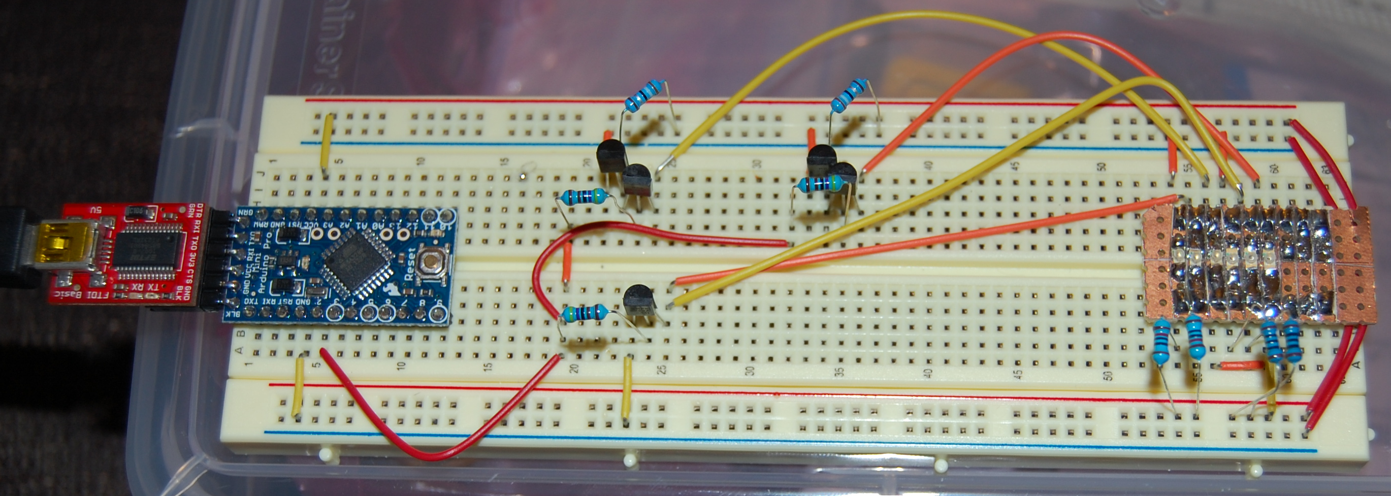
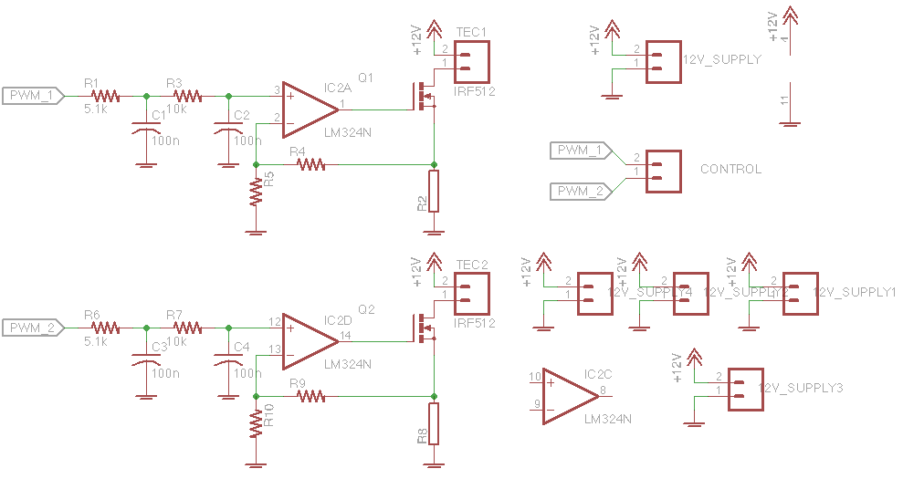
The TEC controller, though, is where things get difficult. Coming from an Arduino, PWM is easy, but TEC efficiency is greatly reduced when controlled in this fashion. To get analog control of TEC current, I designed a PWM-to-constant-current converter board. The basic principle of operation is to use an op-amp, MOSFET, and power resistor to form a feedback-controlled current sink. Then, rather than using a potentiometer to set target current, I’m using the PWM output of an Arduino plugged into an RC lowpass filter. The filter converts the PWM into an analog voltage, which is converted into the target current by the op-amp feedback network.

Simple enough scheme, but unfortunately I still had to go through a few revisions.

In rev 1, I made a ~~small~~ order of magnitude math error and incorrectly sized my power resistor, thus dissipating about 10x my desired wattage in the resistor. (It’s hard to appreciate what it means when these things are rated as “fire proof” until your IR thermometer reads 300 degrees C.)

After correcting that math, it turned out that I had my feedback dividers set in the wrong direction – I actually need to step the input voltage down, not the feedback voltage – so I spun another version of the board. This worked much better, but to my dismay I couldn’t get both the hot and cold channels to reach as much of a temperature difference as I wanted. After some head scratching, I determined that my power supply wasn’t beefy enough to drive two 10A loads at once and must be sagging, so I Amazon’d up a much bigger one. When I plugged that in and let it rip, things looked good until my tragically undersized +12V trace heated up to red-hot and blew like a fuse. In retrospect, of course that trace was too small… but I think I had been telling myself I would solder-fill it or something to increase carrying capacity.

So we’re on to rev 3. This version solves all the problems I’ve come across so far: better connector strategy, better layout for the analog components around the opamp (fewer vias), smaller outline, and of course the fattest power traces I could pull off. I milled it out, riveted the vias, flooded the power traces with solder, and stuffed it full of components. I’m feeling pretty good about this one, but I won’t be able to test it until I get all my plumbing straightened out again.

Mounting brackets

Waterblock, TEC, heatsink mounting bracket

I’m also tired of using zip ties to mount everything to my project board, so I started on the process of making permanent mounting brackets for the important parts.

The first thing up is the hot-side waterblock, TEC, and heatsink. The design is very simple – just a sort of pocket that holds all the parts in a stack and a retainer that slips over the top. There are holes in the corners to bolt it down. This was the first time I’ve ever tried milling such a thick piece of plastic, and I found it be a bit challenging due to the debris evacuation aspects. I used a 1/8″ upcut endmill, which worked fine for the main cavity, but in the continuous, thin, deep cut of the outline, chips accumulated, remelted, and ultimately bogged down the mill. I was able to rescue this part with some cowboy maneuvers, but overall the result wasn’t too great. I’ll be remaking this for sure with better tooling and/or process. I’ll make a similar version that mates with the giant CPU chiller I’m using on the cold side, too.

What’s next

As soon as I have brackets for remounting the main components, I’m going to start on a new project board and try to mount everything closer to what I’ll want it to look like in the final enclosure. Then I’ll transfer all the control electronics to a more permanent breakout board, and start to design the final enclosure. Still lots to do, but definitely inching along!

Designing a capacitive touch wheel in OpenSCAD and EAGLE

4 Replies

I’m a big fan of DIY capacitive touch sensors. Without any custom parts or special fabrication techniques (beyond regular PCB creation), you can create really impressive interfaces. I first used this on the Question Block Lamp (Getting ready to ship! Order yours now!), and ever since I’ve been looking for great places to apply the technique.

Recently, I decided that one of my projects would really benefit from the addition of a capacitive touch wheel. I didn’t want to re-invent the wheel, so to speak, so I started Googling for designs.

The design

The page for the Arduino CapSense library sent me looking for the Quantum Scrollwheel sensor datasheet, which contains a handy schematic for a scroll wheel. So how’s this thing supposed to work? The wheel is composed of three separate, identical electrodes that are tessellated together to form a ring. Each electrode is interleaved with its neighbors such that as you move away from the center of one electrode, the current electrode exposes less and less surface area while the next one exposes more and more. This means that if you measure the capacitance values of all three electrodes in succession, you should see approximately complimentary values on two of them, and an “untouched” value on the third. This should be sufficient information to figure out the orientation of the touch.

Ok, so how do we draw this?

The schematic for this wheel design is straight-forward enough, but this is far from an easy shape to draw. As I highlighted in a previous post, EAGLE really isn’t going to help you draw something like this, so you need to turn to another program to do it and then import the results. My tool of choice is OpenSCAD, so I got to work on a script to generate this shape.

Since all the electrodes are identical, we really only have to draw one and then rotate some copies around to complete the tessellation. Only, this shape is a bit unique – the curved triangular sections don’t lend themselves to being described with simple OpenSCAD primitives.

The first approach I considered was to think of each curved triangle is as a regular 2D triangle, only rendered incrementally along an arc. Polar coordinates would make this especially easy to describe. While this feels like it would be an elegant way to express these sections, OpenSCAD isn’t friendly to this approach. You can define arbitrary polygons, but you can’t add points to a polygon with any sort of native loop. In the past, when I had no other choice, I’ve written a Ruby script to generate the point list manually and then pasted them into my OpenSCAD script. This is clunky and involved, so I try to avoid it if at all possible.

However, I came up with another way to express this shape that is more amenable to being generated directly in OpenSCAD. It’s a technique I found on the OpenSCAD mailing list that the creator referred to as “chain hull”. A chain hull of a list of primitives is the union of the convex hulls of neighboring pairs of said primitives. Did you follow that? This page has a good visual example of the operation in action. I think chain hulling is a brilliant use of the primitive functions available in OpenSCAD and allows for complex shapes to be described very concisely.

To build our curved triangle sections with a chain hull, I laid out an arc of very thin squares ranging from the minimum width to the maximum width in a linear fashion. The chain hull magic takes each pair of squares, hulls them, and then unions all the results. Here’s the code that generates the shape:

	module curved_triangle(r, pitch, separation, gap) {
	assign(num_steps = 36)
	assign(top_d = pitch - 2 * separation)
	assign(bottom_d = triangle_tip_width)
	assign(delta = top_d - bottom_d)
	assign(d_incr = delta / (num_steps-1))
	assign(b_incr=116/(num_steps - 1))
	render()
	for (i=[0:(num_steps-2)]) {
	hull() {
	rotate([0, 0, b_incr * i])
	translate([r, 0, 0])
	square(size=[top_d - d_incr * i, 0.01], center=true);
	rotate([0, 0, b_incr * (i+1)])
	translate([r, 0, 0])
	square(size=[top_d - d_incr * (i+1), 0.01], center=true);
	echo("blah", top_d - d_incr * (i+1));
	}
	}
	}

view raw curved_triangle.scad hosted with ❤ by GitHub

And here’s a view of the intermediate shapes and the resulting chain hull:

The base shapes, and the chain hull that gets drawn around them.

With a module built to create these curved triangles, the rest of the script is glue code to put the triangles in the right places. I wrote one module to generate the concentric/alternating triangles for an entire electrode, and then another module to generate the whole scroll wheel by rotating three electrodes into their proper positions. The final result comes out looking pretty good:

One gotcha I figured out in the course of this project is that EAGLE really doesn’t like to have zero-width lines, even if they’re just describing the outline of a polygon. To account for this, I drew the wheel sections a tiny bit smaller to account for the line width I’d use in EAGLE. This is not unlike accounting for the kerf on a laser cutter, so if you’ve done that before you’ll be familiar.

Getting it into EAGLE

The next step is getting it out of OpenSCAD and into EAGLE. I wrote about using OpenSCAD shapes as board outlines in another post, but this case is a little different. Board outlines can just be simple wires, but polygons need to be closed shapes. The DXFs that come out of OpenSCAD are just collections of segments. I needed a way to convert these segment lists into ordered lists of points that they could be entered with the POLYGON command. So, of course, I wrote a Ruby script to do it.

The operation for converting a set of segments into a ordered list of points is pretty easy. The trick is to think of the list of segments as edges in a graph, and then the objective becomes traversing the graph and outputting a list of connected components. To do this, first I read all the segments into memory, then put them into a map indexed by their start point. Then I pick an arbitrary segment, write its two points to a list, and then use the second point to do a map lookup for the next segment that matches it. This process then repeats with the second point of each segment until we’re back to the start point. This process nets a list of lists of points, each list being a closed polygon. Once all the segments appear in a polygon, we’re done, and from there it’s easy to generate a set of EAGLE commands and write them into a .scr file.

Before I run this generated script from the EAGLE command prompt, I do one hand editing pass to name the polygons so that they are connected to the proper signals in the schematic. With that done, I set the my desired line width to match what I used in the OpenSCAD script, and then load the polygons into EAGLE by running the command “script poly” where poly is the name of the .scr file created in the last step.

When EAGLE renders the polygons, they’ll start out empty with dotted borders. To get them filled in, you need to route connections to them and then run the RATSNEST command. If you’re planning to use the autorouter, a good practice at this point is to use the restrict and keepout layers to defend these polygons. If you cover the electrodes with a polygon in tRestrict or bRestrict layer (depending on whether your electrode is on the top or bottom), then the autorouter will leave it alone when routing other traces. Just make sure to hand-route a connection point through the protective layer, and then the autorouter will be able to take it from there. (tRestrict/bRestrict are just hints to the autorouter and will not trigger design rule warnings. Pretty handy!)

The whole bottom of the board, featuring the the scroll wheel!

Next steps

I just ordered a batch of boards using the scroll wheel described in this post, so when they arrive, I will populate one and get to work on creating a library for easily reading out a position. Stay tuned for a future post!

Simple constant current LED driver

11 Replies

Here’s a simple circuit for driving LEDs at constant current. I like this one because it can be built with a variety of different components based on what you have on hand. I built my version with two 2N2222A transistors and a sense resistor from my resistor kit.

How does it work?

A small current on the CONTROL line causes the DRIVE transistor to switch on and sink through the SENSE resistor. The FEEDBACK transistor only operates when the voltage at the SENSE resistor is greater than its V_BE, or turn-on voltage. When it turns on, it draws some current away from the base of the DRIVE transistor, reducing its gain and causing it to drop more voltage. This negative feedback will cause the whole system to equilibrate such that the SENSE resistor is seeing exactly the FEEDBACK transistor’s V_BE.

Why is this better than a ballast resistor?

You can drive a variety of LEDs with different forward voltages without worrying about changing any of the components (provided that you are comfortable using the same current). The DRIVE transistor will just drop more or less volts as necessary.

Also, if you’re trying to drive some high-current LEDs, you’re more likely to have common transistors that can handle the power dissipation than you are to have high wattage resistors. This makes prototyping and experimentation easier.

Finally, depending on your LEDs and your power supply, you could end up using fewer components by driving multiple LEDs in a string, rather than driving each LED separately.

Sizing components and calculating current and power

LEDs: You can use as many LEDs as you’d like provided that their combined forward voltage is less than the supply voltage minus V_BE.

Power supply: Your input voltage needs to be at least the sum of the forward voltages of your LED string plus the minimum drop across the DRIVE transistor plus the V_BE of your FEEDBACK transistor. Otherwise there won’t be enough voltage to turn on the LEDs.

Transistors: Anything NPN (or N-channel, if you’re using MOSFETs) you have handy has the potential to work. The most important thing to think about is how much voltage you’re expecting it to drop for you and what that means for power dissipation. This transistor will be acting in its linear region, so any voltage it doesn’t pass on from collector to emitter will turn into heat! For instance, let’s use an example of a 12V power supply and two white LEDs with a 3.2V forward voltage. The drive transistor will have to drop 12 V – (2 * 3.2 V + 0.6 V) = 5 V. If your target current is, say, 200 mA, then the transistor will be dissipating 5 V * 0.2 A = 1 watt of power. For some transistors this is no problem, but for others that’s a death sentence. Read your datasheet!

Sense resistor: This resistor sets the amount of current you want to pass through the LEDs. You can compute its value by taking the V_BE of your FEEDBACK transistor and dividing by desired current. For instance, if you’re using a 2n2222A transistor with a V_BE of 0.6 V, and you want to sink 200 mA of current, you would need a 3 ohm resistor. Power dissipation is straight forward, since you know the voltage and the current. Using our existing example, a 3 ohm sense resistor would see 0.6 V * 0.2 A = 0.12 watts. That’s small enough that you can use 1/4 watt resistors from a part kit with little worry.

Over-driving LEDs for brightness

17 Replies

Most of the time when I’m driving an LED, I do it with a simple ballast resistor, and that’s all there is to it. Lately, however, I’ve been working on a few LED matrix projects, and while it’s certainly possible to use the same simple resistor approach, this leads to a very dim display. (Since any given LED’s duty cycle is 1/N max, they appear much dimmer than they normally would.)

The good news is that there’s a straightforward solution to this problem. LEDs have a rated forward current, but they also have a rated peak current, specified at a given pulse width and duty cycle. For instance, these red LEDs are rated for 30mA forward current and 185mA peak in 0.1 ms pulses at 10% duty cycle. Why is this stat useful? As long as you stick to the pulse width and duty cycle parameters, you can intermittently drive an LED at an excess current and get a brighter light without burning it out.

There is a risk in using this setup, though. If for some reason your PWM signal were to lock up in the “high” state, then the pulse width limitations would be exceeded and you’ll probably fry the LED in an instant. This means you need to be especially cautious during development – crashing your microcontroller at the wrong time can be costly!

While the theory of this is straight-forward, I wanted to test how it actually looks in practice before I integrated it into my design. If it was only moderately brighter, I didn’t want to spend the energy (and money) on adding an array of transistors to my board.

My test setup.

I decided to throw together a test setup that would allow me to compare brightness of an LED at its full-on steady current, one PWM’d with a ballast resistor to keep it at its steady current, and one at peak current and PWM’d. This sets up a comparison between the maximum brightness, the brightness of the same LED in a naively driven matrix, and finally the same LED over-driven.

The LEDs I’m using here are surface mount in a 1206 package. Saying that they are very small is an understatement. They are by no means breadboard compatible, so the first step was creating a simple breakout board.

I used a piece of pre-drilled perfboard with a solid copper pour on one side to make the breakout. I marked off a few columns of 6 holes each so that it would span the IC gutter on a breadboard, then cut the piece out with a pair of aircraft snips. Next, I used a utility knife and a straightedge to score the copper and separate the columns from each other, and then did one horizontal stroke to make a grid of 1×3 hole pads.

Detail of the LED breakout board

Next, I soldered two rows of 0.1″ header to the top and bottom of the board for mating with the breadboard. Then, I hand-soldered 6 LEDs, 3 red and 3 green, onto the board. (Judicious use of continuity tester and solder sucker not optional.) Finally, I used a file to chop one corner as an orientation indicator and then cleaned up the rough edges.

To prove that everything was working, I started out by connecting the steady current resistor and probed all the LEDs. Everything lit up fine. With the baseline established, the next step was to set up the PWM signal. According to this page, the Arduino’s built-in analogWrite() PWM runs at about 500Hz, which is too slow for the target pulse width. Since I didn’t need crazy precision or performance here, I decided to quickly write up an Arduino sketch that toggled the output pin manually and used delayMicros() to set the interval. The sketch turned out to be pretty simple:

[gist https://gist.github.com/bryanduxbury/7729613]

To verify that this was giving the output I expected, I hooked up the output pin to my handy DSO Nano. On the first try I ended up with a 996 Hz frequency and good pulse width. The error in the frequency is probably due to the fact that there’s overhead to toggling pins and calling delayMicros(). I suspect I could dial it into precisely 1000 Hz by guess and test on the delay durations, but it’s not that important at this point. In the real production scenario, I’ll be using a hardware timer and it’ll be worth getting it exactly right.

Connecting the PWM output to the second LED was straight forward, though I did add a NPN transistor in between the output pin and the LED so that it could drive all the PWM inputs without any worries about current draw.

The over-driven LED was the most complicated to set up. I plugged the peak current number into an LED resistor calculator, and it told me I needed a 12 ohm, 2 watt resistor. Yikes! I certainly don’t have anything like that on hand. Rather than putting a whole ton of resistors in parallel, I wired up a simple constant current LED driver circuit using some common transistors and resistors. I’ll leave the discussion of that driver circuit for another time, but the cool thing about it is that it allows the transistors to do all the heavy wattage dissipation while the resistors see a tiny load.

With everything wired up, I powered it on to assess the results:

Closeup of the final brightness test. Hooray for DSLR cameras!

I would say that the PWM-only LED is substantially dimmer, and the overdriven LED is almost but not quite as bright as the steady-on LED. This turned out to be exactly the sort of obvious difference I was looking for. It seems well worth adding the additional circuitry to get a much brighter display.

Bryan Duxbury's Blog

Making stuff and taking names. Well, making stuff, anyways.